
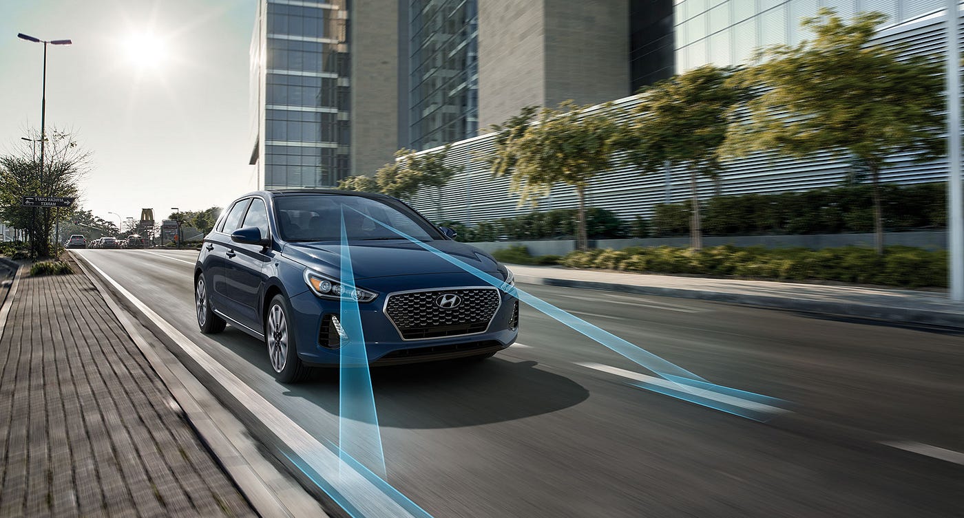
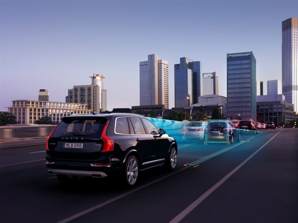
The Automotive industry is currently experiencing a paradigm shift from conventional human-driven vehicles to autonomous self-driving vehicles. With it, Self-driving cars are constantly making the headlines. What seemed like a sci-fi movie decades back, is right now the reality. We now have vehicles that are designed to carry humans from point A to point B without any human intervention. Right now Self Driving cars are one of the hottest areas of research and there is no doubt that self-driving cars are the future!
These self-driving cars use computer vision and deep learning in solving automotive problems, including detecting lane lines, predicting steering angle, and much more.
In this blog, I will teach how to use essential Computer Vision techniques to identify lane lines on a road image/video stream.
Computer Vision for Autonomous Driving
We, humans, are heavily dependent on our five senses to interpret what is going on around us. Every sense is equally important to us. Eyes are what we use to see and perceive a lot of things around us. It helps us to see the road around us, see the obstacle around us, identify the lanes and much more. In applications like autonomous vehicles, robots, this still is one of the most challenging tasks to teach machines to see and understand like humans.
Computer vision is one of the hottest topics in Artificial Intelligence. It is being used extensively in Robotics, Autonomous Vehicles, Image Classification, Object Detection & tracking, Semantic Segmentation as well as in various photo correction apps. In Autonomous vehicles, vision remains the main source of information to detect lanes, traffic lights, and other visual features.
Despite the challenges, we have already done so many advancements in the field of Computer Vision.
Autonomous vehicles like Tesla heavily depend on Camera/Computer vision while it’s competitor depend on Lidar. And I remember this statement Elon Musk on Tesla’s Autonomy day.
“Lidar is Fool’s Errand, Anyone relying on Lidar is doomed! Doomed!! It’s like having a whole bunch of expensive appendices. Like, one appendix is bad, well now you have a whole bunch of them, it’s ridiculous, you’ll see.”
There’s been a lot of debate on which one is better. Recently Lex Fridman (Research Scientist at MIT working on human-centered Artificial Intelligence) was interviewed by Joe Rogan, and I quote this from Joe Rogan Experience #1292
Elon Musk says best sensor is camera, everybody says at this time LIDAR: these lasers are the best sensors. So here’s the difference: Lasers are more precise, they work better in poor lightening conditions, they are more reliable. You can build safe systems today, that use lidar. The problem is that they don’t have much information. So if you are going to build Artificial Intelligence systems or machine learning systems, that learn from huge amount of data, camera is the way to go. You can learn so much more, you can see so much more! So the richer, deeper sensor is camera, But its harder, you have to collect huge amount of data. So today if you have to build a safe system, you can go for LIDAR, tommorow however you define tommorw, Elon Musk says this in a year, other says five, ten, twenty years, camera is the way to go. That’s the hard debate.
Well, Elon and Lex are genius 😉
If you want to know more about computer vision on Autonomous Driving, here is a nice article written on it.
Naturally, one of the first things to do in developing a self-driving car is to automatically detect the lane lines using some sort of algorithm. In this project, we will use Python and OpenCV to automatically identify the lane lines.
OpenCV
OpenCV stands for “Open Source Computer Vision” is a library for computer vision and machine learning software library invented by Intel in 1999. OpenCV has C++, Python, Java and MATLAB interfaces and supports Windows, Linux, Android, and Mac OS. OpenCV has been written natively in C++ and has a templated interface that works seamlessly with STL containers.

OpenCV Installation
You can install OpenCV using pip package installer.
pip install opencv-python
The detailed installation steps can be found here as well.
OpenCV-python installation
Verifying OpenCV Installation
After the installation, try importing the package to make sure if everything is working fine.
import cv2
cv2.__version__
If everything works perfectly fine, without any errors, you are good to go!
Oh yes, I should not forget to mention Google Colab! If you are somebody who hates installing everything, and just want to code, Google Colab is what you are looking for! And you know? GPU!!! Google Colab provided FREE GPU!!! What else do you need? 😉
You can try these stuffs on https://colab.research.google.com. Give it a try, It’s awesome! OpenCV comes preinstalled on Google Colab 😉
Lane line detection using OpenCV
Loading the Image Frame and defining the Region of Interest
The purpose of this section is to build a program that can identify lane lines in a picture or a video frame. When we humans drive, we use eyes and common sense to drive. We can easily identify the lanes on the road, and we do the steering based on that. But to do this with machines, it’s a difficult task and that’s when computer vision comes in. We build complex computer vision algorithms in order to teach machines to identify the lane lines.
Our main approach here is to build a sequence of functions in order to detect lane lines. We will use an image frame as a sample image, once we are able to detect lane lines in this image frame then we will club everything together which can accept dash cam video footage and detect lane lines on it.
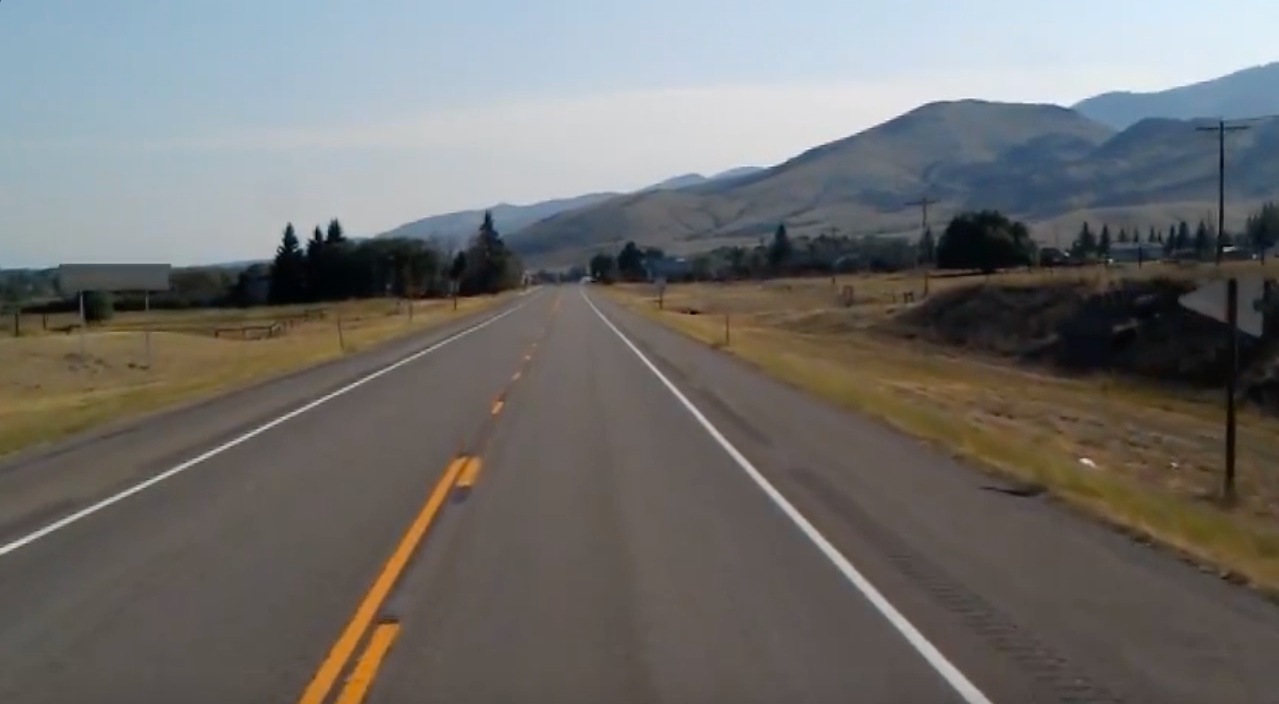
We will start with this image frame:
Loading this image and converting it into grayscale.
Loading image in OpenCV is pretty straightforward
import cv2
lane_image = cv2.imread('road.jpeg')
The reason why we have to convert this image to grayscale is that Processing a single channel is much faster than 3 channel RGB and is less computational intense. A colorful image would have 3 channels, Red, Green, and Blue. Each pixel would have intensities for 3 colors. But that in GrayScale would have the intensity for just one color ranging from 0 to 255.
Let’s convert it to grayscale.
gray = cv2.cvtColor(lane_image, cv2.COLOR_RGB2GRAY)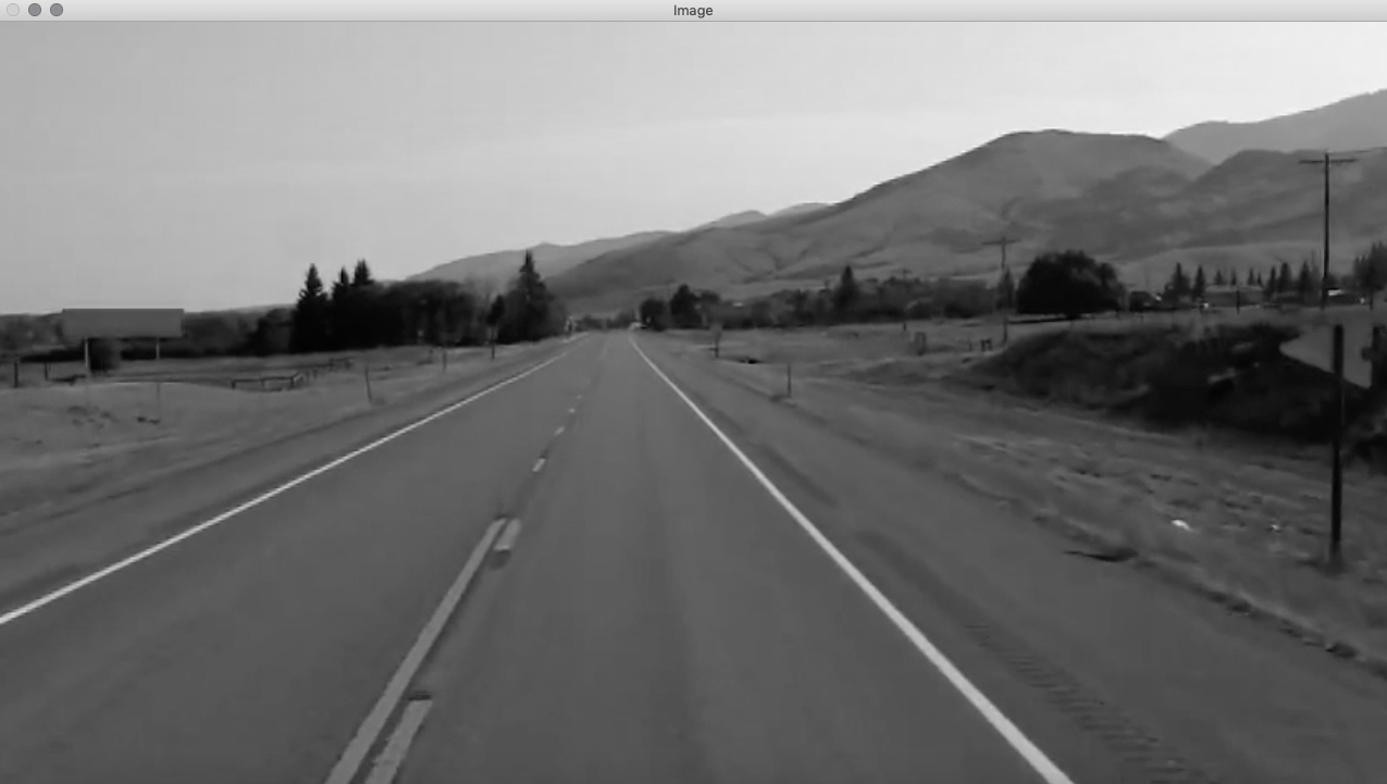
Reduce Noise and Smoothen Image
This image consists of Noise and we need to remove them. Noise can be removed by blurring it. Image Noise creates false edges and can ultimately affect edge detection which is a very crucial step in lane line detection. There could be many reasons for blurring, but here we will use it to reduce the noise. We will use the Gaussian Filter to blur the image. A Gaussian filter nonuniform low pass filter.
Here we want to blur the above gray image using a 5 X 5 kernel.
blur = cv2.GaussianBlur(gray, (5,5), 0)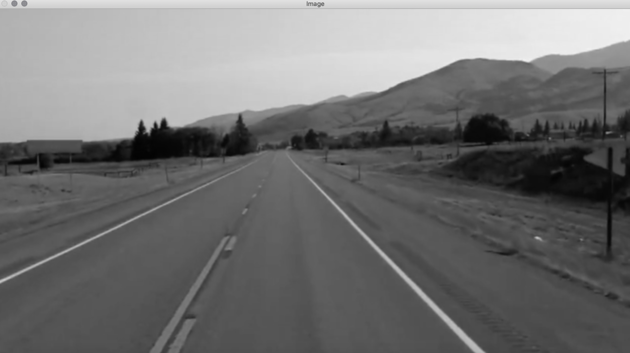
Note: The kernel height and width must be a positive and odd number.
You may increase or decrease the Kernel Height and Width to see the change in intensity of Blur.
In OpenCV using Gaussian Filter is pretty straightforward, but tweaking the parameters requires the understanding of the mathematics of image noise.
Edge Detection (Canny)
Canny Edge detection is one of the widely used Edge Detection Algorithm. Developed by John Canny in 1986, it is a multi-stage algorithm for edge detection. The various stages of Canny Edge Detection algorithm are:
1. Noise Reduction
2. Finding Intensity Gradient of Image

3. Non-Maximum Suppression
4. Hysteresis Thresholding
Canny Edge function also implements 5 X 5 Kernel Gaussian Filter that we used in the previous step. Even though Canny has it’s own function for removing noise, it is advised to implement your own Blurring Function before Canny Edge Detection.
We call that an edge is a region in an image where there is a sharp change in intensity or sharp change in the color between an adjacent pixel in the image. The change in brightness over a series of the pixel is a gradient. A strong gradient indicates steep change and a small gradient indicates a shallow change. Wherever there is an edge, the adjacent pixels on either side of edge have a big difference between their intensities. The image is first scanned in both horizontal and vertical direction to find a gradient for each of the pixel. After getting gradient magnitude and direction, a full scan of an image is done to remove any unwanted pixels which may not constitute the edge. For this, at every pixel, the pixel is checked if it is a local maximum in its neighborhood. This step is called Non-Maximum Suppression.
canny = cv2.Canny(image, low_threshold, upper_threshold)
low_threshold and upper_thresholddetermine how strong the edge must be to be detected.
Recommended low to high threshold ratio is 1:2 or 1:3
cannyImage = cv2.Canny(blur, 50, 150)
Now that we have computed the strongest gradient, we need to define our region of interest.
Before that, let’s put this all together.
def CannyEdge(image):
  gray = cv2.cvtColor(image, cv2.COLOR_RGB2GRAY)
  blur = cv2.GaussianBlur(gray, (5,5), 0)
  cannyImage = cv2.Canny(blur, 60, 180)
  return cannyImage
Region of Interest
For us,
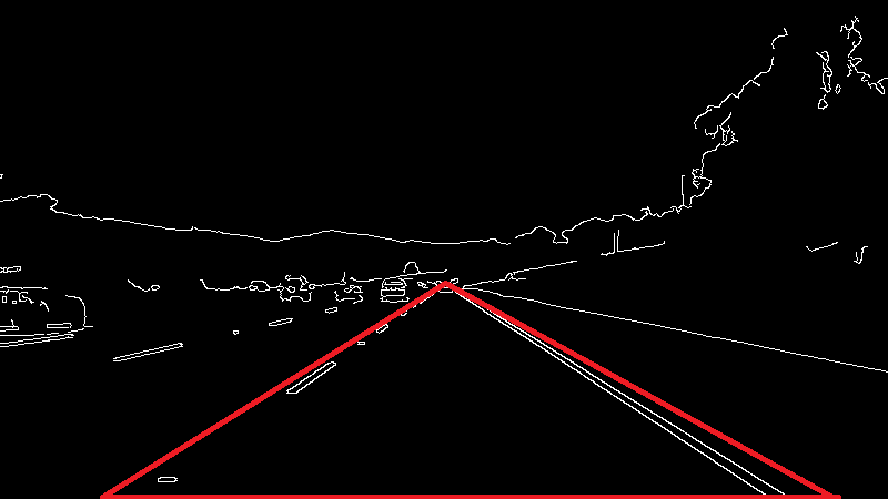
The area inside this red triangle is the region of our interest. We need the coordinates of these points to define our region of interest. To find the coordinates, we can use matplotlib.
import matplotlib.pyplot as plt
plt.imshow(CannyEdge(image))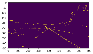
Now we know the coordinates of our region of Interest. Let’s create a function called region_of_interest which takes one argument called image.
def region_of_interest(image):
  height = image.shape[0]
  triangle = np.array([[(200, height),(550, 250),(1100, height),]], np.int32)
  mask = np.zeros_like(image)
  cv2.fillPoly(mask, triangle, 255)
  return mask
This is what exactly our mask looks like. Let me explain to you what we just did.
In the variable triangle, we defined a numpy array with vertices of our masked triangle. We know an image is an array of pixels, zeros_like creates an array of zeros with the same shape as the image. Meaning that both mask and row are going to have the same number of rows and columns. Although the mask is going to be completely black because it only contains zeros. We now need to fill our mask with the triangle we just defined which contains the vertices for the field of view. We use OpenCV’s fillPoly function in order to fill the polygon on the mask. The third parameter in fillPoly is color of polygon.
But this is not going to make any sense. We need to have lane lines visible. To do this we can use bitwise and operation between the canny image we had and the mask. You know that the result of Binary 1 is 1 only when both are 1. As you already know the white pixels in cannyImage and the maskImage both corresponds to 1. So when we do AND operation on both, we get the lane line on our region of Interest. For this, let’s modify our above function slightly.
def region_of_interest(image):
    height = image.shape[0]
    triangle = np.array([[(200, height),(550, 250),(1100, height),]], np.int32)
    mask = np.zeros_like(image)
    cv2.fillPoly(mask, triangle, 255)
    masked_image = cv2.bitwise_and(image, mask)
    return masked_image
This modification is self-explanatory. We just did the AND operation using OpenCV’s bitwise_and(). This is the obtained result.
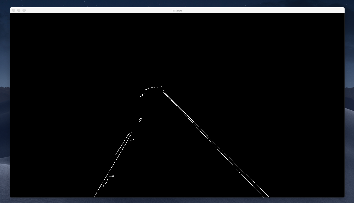
If you compare the image we had got earlier using Canny Edge Detection and this, we have progressed much. Now we have already defined a region of Interest and removed anything else that we do not need.
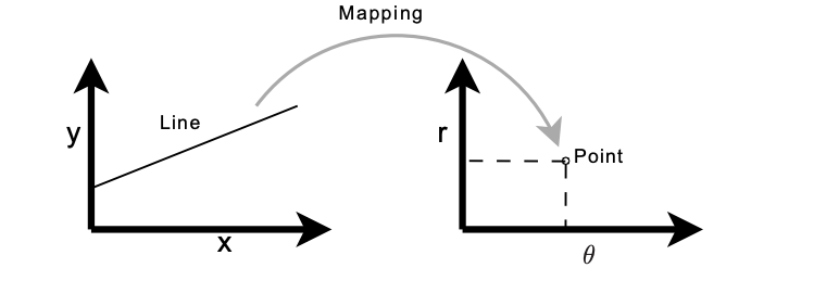
Line Detection — Hough Transform
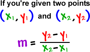
Usually, lines can be represented uniquely by two parameters.
y = m * x + b
This, however, is not able to represent vertical lines. Therefore Hough transform uses an equation
r = x * cos θ + y *sin θ
which in turn can be rewritten in

The Hough space for lines has, therefore, these two dimensions; θ and r, and a line is represented by a single point.
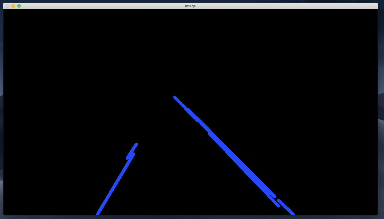
Let’s do this in OpenCV
def display_lines(image, lines):
    line_image = np.zeros_like(image)
    if lines is not None:
        for line in lines:
            x1, y1, x2, y2 = line.reshape(4)
            cv2.line(line_image, (x1, y1), (x2, y2), (255, 0, 0), 10)
    return line_imagecropped_Image = region_of_interest(canny)
rho = 2
theta = np.pi/180
threshold = 100
lines = cv2.HoughLinesP(cropped_Image,rho, theta, threshold, np.array ([]), minLineLength=40, maxLineGap=5)
line_image = display_lines(lane_image, lines)
cv2.imshow('Lane Lines', line_image)
This is what we get,
Now if we want to display these lines on top of our image, we can use an addWeighted function in OpenCV.
combo_image = cv2.addWeighted(lane_image, 0.8, line_image, 1, 1)
cv2.imshow(“Image”, combo_image)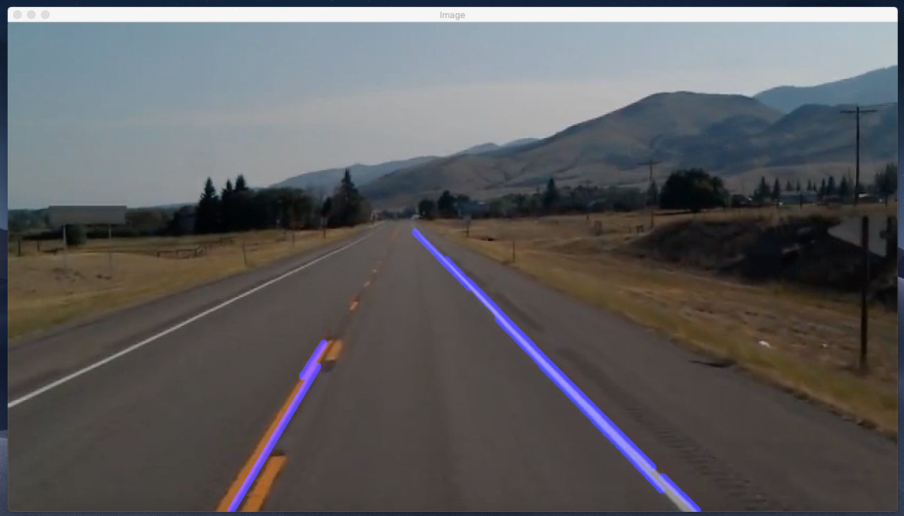
Finally, we got the lines overlayed on top of our lane image.
Let’s do this on video footage. A video is just a collection of multiple image frames.
Slight changes on code,
cap = cv2.VideoCapture("test.mp4")
while(cap.isOpened()):
    _, frame = cap.read()
    canny = CannyEdge(frame)
    cropped_Image = region_of_interest(canny)
    rho = 2
    theta = np.pi/180
    threshold = 100
    lines = cv2.HoughLinesP(cropped_Image,rho, theta, threshold, np.array ([ ]), minLineLength=40, maxLineGap=5)
    line_image = display_lines(frame, lines)
    combo_image = cv2.addWeighted(frame, 0.8, line_image, 1, 1)
    cv2.imshow("Image", combo_image)
    if cv2.waitKey(1) & 0xFF == ord('q'):
        break
cap.release()
cv2.destroyAllWindows()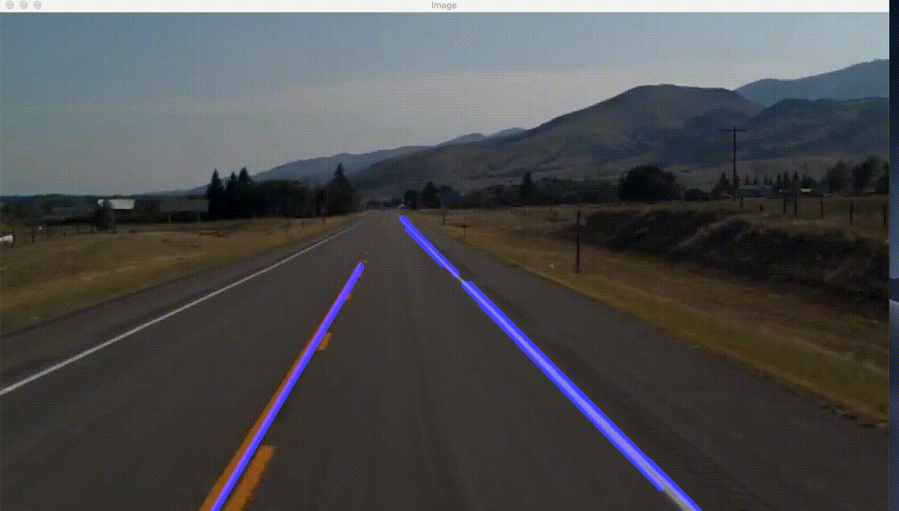
Complete Code
import cv2
import numpy as np


def CannyEdge(image):
  gray = cv2.cvtColor(image, cv2.COLOR_RGB2GRAY)
  blur = cv2.GaussianBlur(gray, (5,5), 0)
  cannyImage = cv2.Canny(blur, 50, 150)
  return cannyImage

def region_of_interest(image):
    height = image.shape[0]
    triangle = np.array([[(200, height),(550, 250),(1100, height),]], np.int32)
    mask = np.zeros_like(image)
    cv2.fillPoly(mask, triangle, 255)
    masked_image = cv2.bitwise_and(image, mask)
    return masked_image

def display_lines(image, lines):
    line_image = np.zeros_like(image)
    if lines is not None:
        for line in lines:
            x1, y1, x2, y2 = line.reshape(4)
            cv2.line(line_image, (x1, y1), (x2, y2), (255, 0, 0), 10)
    return line_image

cap = cv2.VideoCapture("test.mp4")
while(cap.isOpened()):
    _, frame = cap.read()
    canny = CannyEdge(frame)
    cropped_Image = region_of_interest(canny)
    rho = 2
    theta = np.pi/180
    threshold = 100
    lines = cv2.HoughLinesP(cropped_Image,rho, theta, threshold, np.array ([ ]), minLineLength=40, maxLineGap=5)
    line_image = display_lines(frame, lines)
    combo_image = cv2.addWeighted(frame, 0.8, line_image, 1, 1)
    cv2.imshow("Image", combo_image)
    if cv2.waitKey(1) & 0xFF == ord('q'):
        break
cap.release()
cv2.destroyAllWindows()
What we will do now is further optimize how these lines are displayed. As we can clearly see we have multiple lines, what we do now, is we average those lines and obtain a single line.
def average_slope_intercept(image, lines):
    left_fit = []
    right_fit = []
    for line in lines:
        x1, y1, x2, y2 = line.reshape(4)
        parameters = np.polyfit((x1, y1), (x2, y2), 1)
        slope = parameters[0]
        intercept = parameters[1]
        if slope < 0:
            left_fit.append((slope, intercept))
        else:
            right_fit.append((slope, intercept))
    left_fit_average = np.average(left_fit, axis = 0)
    right_fit_average = np.average(right_fit, axis = 0)
What we did here in this function was, we declared two empty lists left_fit and right_fit. left_fit will contain the coordinates of the lines on the left and right_fit will contain the coordinates of the lines on the right. We then iterated through every line, and reshape every line into a one-dimensional array and unpacked into x1, y1, x2, y2.
This x1, y1, x2, y2 are the points of a line and when you are given the point of a line, it is very easy to calculate the slope for an equation y = mx + b.
What polyfit will do it, it will fit a first-degree polynomial, which would be a linear function of y = mx + b; it’s going to fit the polynomial to x & y points and return and vector coefficient of slope in y-intercept.
See: https://docs.scipy.org/doc/numpy/reference/generated/numpy.polyfit.html
One thing to notice is, all the detected road lines on the left are slanted towards the right and detected road lines on the right are slanted towards left. Now if we are to calculate the slope, we will find out that the slope of the detected lines on left will be negative and that on the right will be positive. So we then wrote a condition to check if the slope is towards left or right. And then we averaged all the left_fit and right_fit using a function called average in numpy.
We now need coordinates for our lines, so we made a function called make_points() which returns the coordinates for our lines.
def make_points(image, line_parameters):
    slope, intercept = line_parameters
    y1 = int(image.shape[0])
    y2 = int(y1*3/5)
    x1 = int((y1 - intercept)/slope)
    x2 = int((y2 - intercept)/slope)
    return [[x1, y1, x2, y2]]
What we did here was,
y1 = int(image.shape[0])
y2 = int(y1*3/5)
We want the length of our lines from the bottom of the image to 3/5th of the total image height. And similarly, we calculated the x co-ordinates as well using the slope.
x1 = int((y1 - intercept)/slope)
x2 = int((y2 - intercept)/slope)
Now, the complete average_slope_intercept() function looks like this, nothing much changed but added a line to return the array of lines.
def average_slope_intercept(image, lines):
    left_fit = []
    right_fit = []
    for line in lines:
        x1, y1, x2, y2 = line.reshape(4)
        parameters = np.polyfit((x1, y1), (x2, y2), 1)
        slope = parameters[0]
        intercept = parameters[1]
        if slope < 0:
            left_fit.append((slope, intercept))
        else:
            right_fit.append((slope, intercept))
    left_fit_average = np.average(left_fit, axis = 0)
    right_fit_average = np.average(right_fit, axis = 0)
    return np.array((left_line, right_line))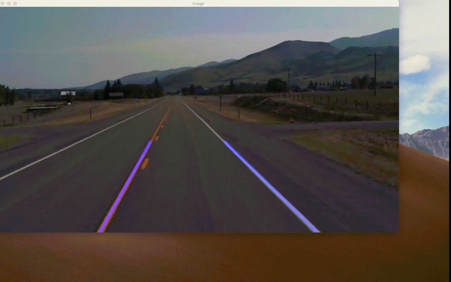
Final Code
import cv2
import numpy as np

def make_points(image, line_parameters):
    slope, intercept = line_parameters
    y1 = int(image.shape[0])
    y2 = int(y1*3/5)
    x1 = int((y1 - intercept)/slope)
    x2 = int((y2 - intercept)/slope)
    return [[x1, y1, x2, y2]]

def average_slope_intercept(image, lines):
    left_fit = []
    right_fit = []
    if lines is None:
        return None
    for line in lines:
        x1, y1, x2, y2 = line.reshape(4)
        parameters = np.polyfit((x1, x2), (y1, y2), 1)
        slope = parameters[0]
        intercept = parameters[1]
        if slope < 0:
            left_fit.append((slope, intercept))
        else:
            right_fit.append((slope, intercept))
    left_fit_average = np.average(left_fit, axis = 0)
    right_fit_average = np.average(right_fit, axis = 0)
    left_line = make_points(image, left_fit_average)
    right_line = make_points(image, right_fit_average)
    return np.array((left_line, right_line))


def CannyEdge(image):
  gray = cv2.cvtColor(image, cv2.COLOR_RGB2GRAY)
  blur = cv2.GaussianBlur(gray, (5,5), 0)
  cannyImage = cv2.Canny(blur, 50, 150)
  return cannyImage

def region_of_interest(image):
    height = image.shape[0]
    triangle = np.array([[(200, height),(550, 250),(1100, height),]], np.int32)
    mask = np.zeros_like(image)
    cv2.fillPoly(mask, triangle, 255)
    masked_image = cv2.bitwise_and(image, mask)
    return masked_image

def display_lines(image, lines):
    line_image = np.zeros_like(image)
    if lines is not None:
        for line in lines:
            x1, y1, x2, y2 = line.reshape(4)
            cv2.line(line_image, (x1, y1), (x2, y2), (255, 0, 0), 10)
    return line_image


cap = cv2.VideoCapture("test.mp4")
while(cap.isOpened()):
    _, frame = cap.read()
    canny = CannyEdge(frame)
    cropped_Image = region_of_interest(canny)
    rho = 2
    theta = np.pi/180
    threshold = 100
    lines = cv2.HoughLinesP(cropped_Image,rho, theta, threshold, np.array ([ ]), minLineLength=40, maxLineGap=5)
    averaged_lines = average_slope_intercept(frame, lines)
    line_image = display_lines(frame, averaged_lines)
    combo_image = cv2.addWeighted(frame, 0.8, line_image, 1, 1)
    cv2.imshow("Image", combo_image)
    if cv2.waitKey(1) & 0xFF == ord('q'):
        break
cap.release()
cv2.destroyAllWindows()
In the next blog, I will try to put everything together, install opencv in raspberry pi and make a small prototype car that can identify the lane lines and navigate. Stay tuned 😉