Machine learning is right now the hottest thing. Every business wants to deploy a machine learning model for their business case. It has given us intelligent robots, self-driving cars, virtual personal assistants like Siri and Google assistant, etc. Remember buying something a couple of days back and you keep getting shopping suggestions or recommendations based on your recent purchase? Or maybe, have you any day got a notification from Facebook saying “Your friend added a photo that might include you!”

It’s machine learning that makes all these possible. But at the heart of all this, is the Data! Data plays a crucial role in the journey of making a machine learning model. Your sophisticated machine learning applications can’t be built on top of poor data.

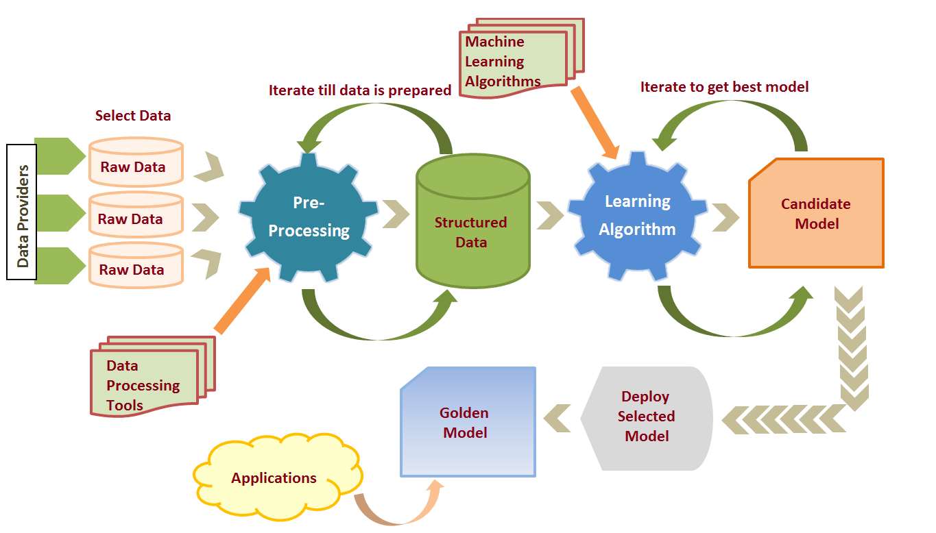
Before raw data could be sent through a machine learning model it has to undergo preprocessing. And it’s simply because data in the real world are generally Incomplete, Noisy and Inconsistent. And if this is fed into the machine learning model, results can come unexpectedly! And that’s not really what we want. Data preprocessing is a proven method for resolving such issues.

Okay! So how data preprocessing is done?

Data preprocessing is generally carried out in 7 simple steps:

1. Gathering the data
2. Import the dataset & Libraries
3. Divide the dataset into Dependent & Independent variable
4. Check for missing values
5. Check for Categorical values
6. Split the dataset into training and test set
7. Feature Scaling

Gathering the data

Data is raw information, its the representation of both human and machine observation of the world. Dataset entirely depends on what type of problem you want to solve. Each problem in machine learning has its own unique nuance and approach. And sometimes it can be quite hard to find the specific dataset for the variety of machine learning problems. But the good news is, there is dataset for every problem you can think of. Here is the curated list of websites you can get the datasets from:

1. Kaggle: Kaggle is my personal favorite one to get the dataset.
   https://www.kaggle.com/datasets
2. UCI Machine Learning Repository: One of the oldest sources of datasets on the web, and a great first stop when looking for interesting datasets.
   http://mlr.cs.umass.edu/ml/
3. This super awesome GitHub repo has tons of links to the high-quality datasets.
   From their GitHub readme: This list of topic-centric public data sources in high quality. They are collected and tidied from blogs, answers, and user responses. Most of the data sets listed below are free, however, some are not.
   Link: https://github.com/awesomedata/awesome-public-datasets
4. There is this Zanran Numerical Data Search Engine too! http://www.zanran.com/q/
5. And if you are looking for Government’s Open Data then here is few of them:
   Indian Government: http://data.gov.in
   US Government: https://www.data.gov/
   British Government: https://data.gov.uk/
   France Government: https://www.data.gouv.fr/en/
6. And of course Google search!

Please do visit this Quora question: https://www.quora.com/Where-can-I-find-large-datasets-open-to-the-public
It’s worth reading.

Here is the dataset I downloaded and will be using from Kaggle “Top Spotify Tracks of 2018 — Audio features of top Spotify songs”.
You can download it from https://www.kaggle.com/nadintamer/top-spotify-tracks-of-2018
This is how the dataset looks like

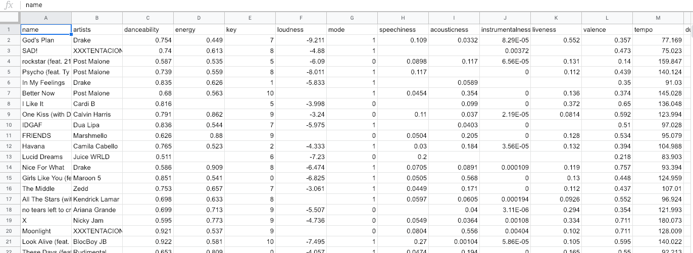
Now I have deliberately removed some values to show how to handle missing values. Remember, I told you real-world data are Incomplete, Noisy and Inconsistent? This is how it may look like in general.

If you observe carefully there are empty cells, those are deliberate. You will see how to play with this soon.

Once you are done with selecting the data, the next step would be to import the required libraries and dataset.

Import the dataset & Libraries

Now let us import the dataset and libraries.

Libraries are collections of modules that can be called and used. They are collections of functions and methods that allow you to perform lots of actions without writing your own code. There are lots of libraries that you would need during this process. I will import and explain it to them when needed.

But there are few libraries in Python for data science and machine learning that you don’t want to miss out!

1. Numpy: NumPy is an extensive library for data storage and calculations. This library contains data structures, algorithms, and other things that are used to handle numerical data in Python.
2. Pandas: Pandas is a powerful and easy to use data structure and data analysis toolkit. Here we will be using pandas for importing the dataset and playing with it.
3. matplotlib: matplotlib is used for data visualization.

4. scikit-learn: This is probably the most used library for machine learning. scikit-learn is a huge library of data analysis features. scikit-learn is used to build models. It should not be used for reading the data, manipulating and summarizing it. It consists of Supervised learning algorithms, cross-validation, unsupervised learning algorithms, feature extraction etc.

How to import the dataset?

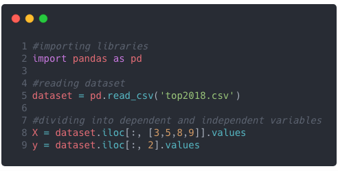
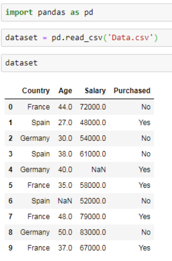
We will use pandas to read the dataset, the one we downloaded from Kaggle in CSV format.

Quite simple, isn’t it? You can do much more like you can know the shape, read first n rows, read last n rows etc.
Let’s try out these!

dataset.shape
> (100, 14)#some times its a good idea to show few rows of data than to flood your screen with entire rowsdataset.head(5)
>
     name       artists     ...         tempo  duration_ms
0                    God's Plan         Drake     ...        77.169       198973
1                          SAD!  XXXTENTACION     ...        75.023       166606
2    rockstar (feat. 21 Savage)   Post Malone     ...       159.847       218147
3  Psycho (feat. Ty Dolla $ign)   Post Malone     ...       140.124       221440
4                In My Feelings         Drake     ...        91.030       217925[5 rows x 14 columns]

Also if you wanted to know the last few rows, use tail

dataset.tail(2)
> .  name     artists     ...         tempo  duration_ms
99  Be Alright  Dean Lewis     ...       126.684       196373[1 rows x 14 columns]

Or if you wish to know only columns

dataset.columns
>
Index(['name', 'artists', 'danceability', 'energy', 'key', 'loudness', 'mode',
       'speechiness', 'acousticness', 'instrumentalness', 'liveness',
       'valence', 'tempo', 'duration_ms'],
      dtype='object')

Divide the dataset into Dependent & Independent variable

After importing the dataset, the next step would be to identify the independent variable (x) and the dependent variable (y). Let’s go back to high school mathematics and try to remember what are these?

An independent variable (x) is a variable that you purposely change in order to see the effect in the dependent variable(y).
For example, in equation y = mx + c, x is the independent variable and y is the dependent variable because you change/tune x to see its change on y. Isn’t it?

In the real world, consider a scientist who wishes to study the impact of a drug on cancer. The independent variables are timing of drug, dosage, etc. Where as dependent variable is the impact. If he/she wishes to see the change in impact of drug, he/she may tune/change the timing and dosage.

In our case, if we wish to predict the danceability based on energy, loudness, acoustics & instrumentalness, our dependent variable (y) would be danceability and independent variable would be energy, loudness, acoustics & instrumentalness.

So let’s do that! To do this we need iloc from pandas. iloc is integer-location based indexing for selection by position. Confused again? Let’s see the syntax.

iloc[<row-selection>, <column-selection>]

Quick Note:
: selects all, using [] helps you select multiple columns or rows

This is how we were able to select the dependent variable (y) and the independent variable (x).

You must be already feeling a mathematics wizard 😜 I get that 😉

Wait,

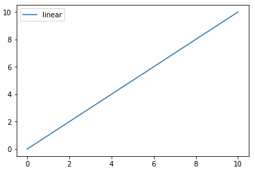
before we move on, remember the matplotlib library we talked earlier? Why don’t we plot a chart based on the dataset to see which artist’s song is more danceable? 😍 Let’s do this!

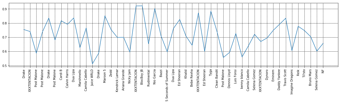
And here is the code for this 😉 Feel free to customize!

Check for missing values

Understanding the ways to manage missing values is very important. As we discussed earlier, real-world data can often have missing values. If the missing values are not handled properly then the researcher may end up drawing incorrect references about the data. And handling the missing values is important because many machine learning models do not support data with missing values.

We can always count the number of columns with missing values.

dataset.isNan().sum()
> dataset.isnull().sum()
name                0
artists             0
danceability        0
energy              2
key                 0
loudness            4
mode                0
speechiness         5
acousticness        3
instrumentalness    2
liveness            4
valence             0
tempo               0
duration_ms         0
dtype: int64

You can see the columns count with missing values. Now there could be two approaches for this:
1. Remove the row completely with missing values
2. Impute missing values
> Impute (replacing missing data with substituted values)

Remove the row completely with missing values

This approach is probably the simplest one but has its trade-off. This can be quite dangerous, what if this row contains crucial information?

It’s not that we never remove the row completely when the value is missing, we do remove it. Like in our dataset, what if the artist name is missing or any class label, you may delete in such case. Also if the missing values columns are neither independent variable nor a dependent variable, it’s better to ignore it.

Pandas provide a dropna() function that can be used to drop either row or columns with missing data. We can use dropna() to remove all the rows with missing data.

dataset.shape
> (49, 14)dataset.dropna(inplace=True)
>dataset.shape
> (38, 14)

You can see that it removed all the rows with missing values. But this is not always a good idea.

Impute missing values

Now, this approach can be applied to a feature that has numeric data like salary, age, etc but not limited to these. We can calculate either mean, mode or median of the feature and replace it with missing values. This is an approximation that can add variance to the dataset.

Now I will use simpleImputer to replace missing data with mean/median/most_frequent.

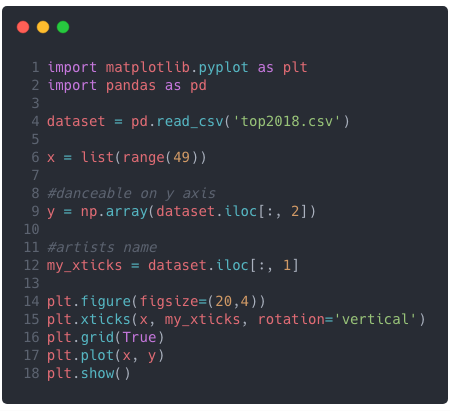
Let’s check our independent variable(x)

import numpy as np
import matplotlib.pyplot as plt
import pandas as pd
from sklearn.impute import SimpleImputer#reading dataset
dataset = pd.read_csv('top2018.csv')#dividing into dependent and independent variables
X = dataset.iloc[:, [3,5,8,9]].values
y = dataset.iloc[:, 2].valuesimputer = SimpleImputer(missing_values=np.nan, strategy="median")
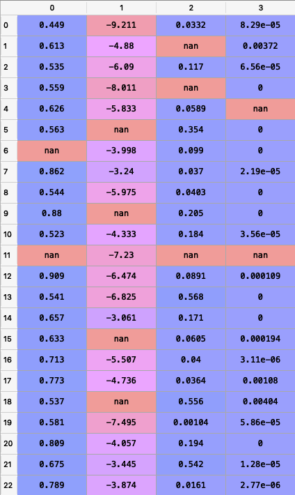
X[:, 0:4] = imputer.fit_transform(X[:, 0:4])

We used median strategy to replace missing values

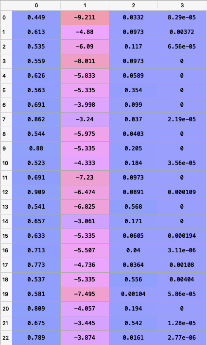
You can see that missing values are replaced by the median strategy. SimpleImputer provides other strategies as well:
1. Constant
2. most_frequent
3. mean
4. median

Now the next question might be when should you use these different approaches? Using these approaches totally depends on the nature of data and the reasons for missing.

Check for Categorical values

Now let’s see how to deal with categorical values.

Sometimes our data can be in the qualititive form, that means we have texts in our data. Now it gets complicated for machines to understand a text and process them rather than numerical values because machine learning models are based on mathematical equation! So there is a need to encode the categorical values.

Our dataset is quite larger and might be difficult to understand. Let’s have a look at this.

As you can see the first column contains data in text form. We can observe that there are 3 categories, France, Spain & Germany. To convert categorical values into numerical data we can use LabelEncoder() class from sklearn.preprocessing.

Let’s import the library

from sklearn.preprocessing import LabelEncoder

The next step would be to create an object of that class, let’s call it labelEncoderX

labelEncoderX = LabelEncoder()

Now to convert this into numerical we can use

X[:,0] = labelencoder_X.fit_transform(X[:,0])

This will select all the rows and 0th column which is countries list and fit the label encoder to it and transform the values. This will be immediately encoded to 0,1,2,3… etc.

print(X)
array([[0, 44.0, 72000.0],
       [2, 27.0, 48000.0],
       [1, 30.0, 54000.0],
       [2, 38.0, 61000.0],
       [1, 40.0, 48000.0],
       [0, 35.0, 58000.0],
       [2, 27.0, 52000.0],
       [0, 48.0, 79000.0],
       [1, 50.0, 83000.0],
       [0, 37.0, 67000.0]], dtype=object)

As you can see the categorical values has been encoded. But there’s a problem!

The problem is still the same. Machine learning models are based on equations and it’s good that we replaced the text by numbers. However, since 1 is greater than 0 and 2 is greater than 1 the equations in the model will think that Spain has a higher value than Germany and France and Germany has a higher value than France. And that’s certainly not the case. These are actually three categories and there is no relational order between these three. We cannot compare France, Spain, and Germany by saying that Spain is greater than Germany or Germany is greater than in France.

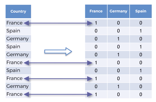
So we need to find a way to prevent the machine learning equations from thinking Spain is greater than Germany and Germany is greater than France. To prevent this we use Dummy variables.

What are the Dummy variables?

Dummy variables are discrete variables taking values of either ‘0’ or ‘1’. They are often called ‘On or Off’ variables or indicator variables. They just take 0 or 1 to indicate the presence of a categorical effect.

Instead of having one column and assigning a numerical value which might cause bias, we create different columns based on the type of categories present.
Number of Columns = Types of Categories

In our case we have 3 types, so we are going to have 3 columns. To do this we will import yet another library called OneHotEncoder.

from sklearn.preprocessing import LabelEncoder, OneHotEncoder

Next step is to create an object of that class with an important parameter called categorical_features which takes a value of the index of the column.

onehotencoder = OneHotEncoder(categorical_features =[0])

Just how we used fit_transform() for LabelEncoder we will use for OneHotEncoder as well.

X = onehotencoder.fit_transform(X).toarray()

Now if you see our independent variable (X) this is how it looks like.

Split the dataset into Training Set and Test Set

When we take a step back and focus on the word Machine Learning it makes sense that your model is going to learn from your data and make predictions. And when machines do such predictions, we need to validate them as well.

The training dataset is used to train the model. The model learns from this data. And the test set is used to check how accurately our model can predict.

Again we will import a library from scikit called test_train_split from model.selection class

from sklearn.model_selection import train_test_split

We need 4 variables now, X_train, X_test, y_train, y_test.

Let’s divide our dataset into train and test set.

X_train, X_test, y_train, y_test = train_test_split(X,y, test_size=0.2)

test_size + train_size = 1

What we did here was we divided the 20% of data into test set and 80% data into training data. Now there is no rule of thumb as such that you should divide your dataset to 80–20 ratio but its a very common practice.

I had taken Andrew Ng’s online machine learning course. His recommendation was Training: 60% Cross-validation: 20% Testing: 20%.
Now, this is just a recommendation! At the end of the day, It all depends on the data at hand.

Now if you see our dataset of top songs of 2018, this is what happens. We had 50 rows of data, 20% of 50 would be 10, so 40 sets in training and 10 is a test.

Feature Scaling

This is the final step in data preprocessing is the Feature scaling. Feature scaling is the proven method to limit the range of variables so that they can be compared on common grounds. For example, if you see this dataset

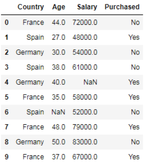
The salary ranges from 48000 to 83000. Similarly, Age ranges from 27 to 50. If you see carefully one feature is measured in tens and other in thousands. Most machine learning algorithms consider only the magnitude of the values, not the units of those values.

Many machine learning algorithms are based on what is called Euclidean Distance.

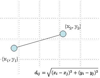
Let’s say if we take the distance between (72000–48000)² = 576000000 & (44–27)² = 289. 576000000 clearly dominates over 289 and we do not that to happen. Now we have to limit the range of variables so that they can be compared on common grounds!

There are several ways of scaling the data. There are two ways you can do this.

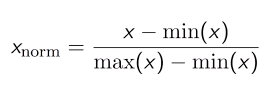
Normalization

Normalization scales the feature between 0.0 & 1.0, retaining their proportional range to each other.

Standardization typically means that the range of values is “standardized” to measure how many standard deviations the value is from its mean. Standardization transforms your data such that the resulting distribution has a mean of 0 and a standard deviation of 1.

To do this we need to import StandardScaler from the scikit preprocessing library

from sklearn.preprocessing import StandardScaler
sc_X = StandardScaler()

Now all we need to do is fit and transform our X_Training set.

Quick Note: For the test set, you must fit and then transform, but for training set simply transform is required.

Now you would see that data will be on the same range.

These were the general steps for preprocessing the data. Depending on the dataset you have, you may or may not need to follow these steps.

Thank you for making it till here! I hope you enjoyed this!

Let’s connect if you are there on LinkedIn Yogesh Ojha

If you have any questions or suggestions, please do let me know 😃

Happy machine learning 🤖

This article was originally published on Medium: https://yogeshojha.com/home1/a-beginners-guide-to-machine-learning-data-preprocessing/